Confidence Regions from Prediction Algorithms#
INTRO & SETTINGS#
The goal of this tutorial is to show the capabilities of lf2i and Waldo with a simple example: inferring the mean \(\theta \in \mathbb{R}\) of a Gaussian model with fixed variance, and a Gaussian prior distribution
In addition, we assume that we only observe one sample for each true \(\theta\), i.e., \(n=1\).
For this tutorial, we leverage a prediction algorithm as the main underlying inferential model.
# SETTINGS

LIKELIHOOD_COV = 0.01
PRIOR_LOC = 0
PRIOR_COV = 0.1

PARAM_DIM = 1
DATA_DIM = 1
BATCH_SIZE = 1  # assume we get to see only one observed sample for each “true” parameter
PARAM_SPACE_BOUNDS = {'low': -1.5, 'high': 1.5}  # a grid of points over [low, high]^(param_dim) is used to construct confidence sets

CONFIDENCE_LEVEL = 0.90
SIMULATE#
Let’s start from the simulator, which is used internally to generate the data needed to
estimate the test statistics;
estimate the critical values; and
diagnose the constructed confidence regions
from lf2i.simulator.gaussian import GaussianMean
simulator = GaussianMean(
    likelihood_cov=LIKELIHOOD_COV,
    prior='gaussian',
    poi_space_bounds=PARAM_SPACE_BOUNDS,
    poi_grid_size=1000,
    poi_dim=PARAM_DIM,
    data_dim=DATA_DIM,
    batch_size=BATCH_SIZE,
    prior_kwargs={'loc': PRIOR_LOC, 'cov': PRIOR_COV}
)
Observations#
For simplicity, let’s use the simulator to get two “observed” samples from the true likelihood: one consistent with the prior (\(\theta^{\star} = 0\)) and one not (\(\theta^{\star} = -1.45\))
import torch

true_param_consistent, true_param_notconsistent = torch.Tensor([0]), torch.Tensor([-1.45])
observed_x_consistent = simulator.likelihood(true_param_consistent).sample(sample_shape=(BATCH_SIZE, ))
observed_x_notconsistent = simulator.likelihood(true_param_notconsistent).sample(sample_shape=(BATCH_SIZE, ))
CONFIDENCE SET by leveraging a PREDICTION ALGORITHM#
Assume we want to do inference on the Gaussian mean by predicting its value given the data. Waldo allows to leverage any prediction algorithm to obtain a confidence region for the parameter of interest that is guaranteed to have the desired level of coverage regardless of
the prior distribution;
the true value of the parameter;
the size of the observed sample
The prediction algorithm can be pre-trained or not. The example below assumes the algorithm (in this case GradientBoosting) has not been trained yet
from lf2i.inference import LF2I
from lf2i.plot.parameter_regions import plot_parameter_region
from lf2i.utils.other_methods import gaussian_prediction_sets
lf2i = LF2I(
    test_statistic='waldo',
    poi_dim=PARAM_DIM,
    estimation_method='prediction',
    estimator='mlp_r',  # simple feed-forward NN for the conditional mean
    cond_variance_estimator='gb_r',  # for the conditional variance
    estimator_kwargs={'hidden_layer_sizes': (40, ), 'alpha': 0.1},
    cond_variance_estimator_kwargs={'n_estimators': 500, 'max_depth': 1}
)
Note that for this example we are using the simulator to obtain training datasets. If one has pre-simulated datasets, they can be given as inputs directly to the inference method.
confidence_region = lf2i.inference(
    x=torch.vstack((observed_x_consistent, observed_x_notconsistent)),
    evaluation_grid=simulator.poi_grid,
    confidence_level=CONFIDENCE_LEVEL,
    simulator=simulator,
    b=10_000, b_prime=5_000
)
Constructing confidence regions ...
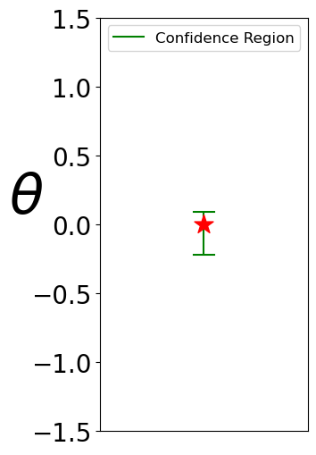
Waldo Confidence Region
# The red star in the plot is the true parameter

plot_parameter_region(
    parameter_region=confidence_region[0],
    param_dim=PARAM_DIM,
    true_parameter=true_param_consistent,
    parameter_space_bounds=simulator.poi_space_bounds,
    figsize=(3, 6)
)
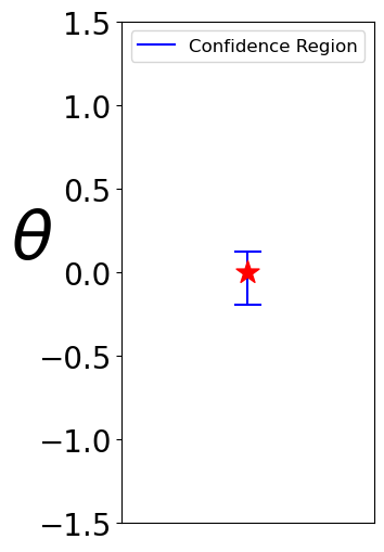
Central (Gaussian approximation) prediction sets
plot_parameter_region(
    parameter_region=gaussian_prediction_sets(
        conditional_mean_estimator=lf2i.test_statistic.estimator,
        conditional_variance_estimator=lf2i.test_statistic.cond_variance_estimator,
        samples=observed_x_consistent,
        confidence_level=CONFIDENCE_LEVEL,
        param_dim=PARAM_DIM
    ),
    param_dim=PARAM_DIM,
    true_parameter=true_param_consistent,
    parameter_space_bounds=simulator.poi_space_bounds,
    color='blue',
    figsize=(3, 6)
)
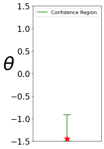
Waldo Confidence Region
plot_parameter_region(
    parameter_region=confidence_region[1],
    param_dim=PARAM_DIM,
    true_parameter=true_param_notconsistent,
    parameter_space_bounds=simulator.poi_space_bounds,
    figsize=(3, 6)
)
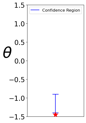
Gaussian prediction intervals centered around the prediction.
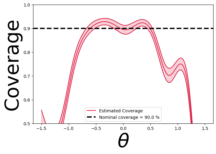
Different observations might give slightly different results, but on average this method does not provide the correct level of coverage (see Diagnostics below)
plot_parameter_region(
    parameter_region=gaussian_prediction_sets(
        conditional_mean_estimator=lf2i.test_statistic.estimator,
        conditional_variance_estimator=lf2i.test_statistic.cond_variance_estimator,
        samples=observed_x_notconsistent,
        confidence_level=CONFIDENCE_LEVEL,
        param_dim=PARAM_DIM
    ),
    param_dim=PARAM_DIM,
    true_parameter=true_param_notconsistent,
    parameter_space_bounds=simulator.poi_space_bounds,
    color='blue',
    figsize=(3, 6)
)
DIAGNOSTICS#
from lf2i.plot.coverage_diagnostics import coverage_probability_plot
Note that for this example we are using the simulator to obtain training dataset. If one has pre-simulated dataset, it can be given as input directly to the diagnostics method.
diagnostic_estimator, parameters, mean_proba, upper_proba, lower_proba = lf2i.diagnostics(
    region_type='prediction',
    simulator=simulator,
    b_double_prime=10_000,
    evaluation_grid=simulator.poi_grid.reshape(-1, PARAM_DIM),
    confidence_level=CONFIDENCE_LEVEL
)
Coverage is close to the correct level (\(90%\)) only when the true parameter is close to the bulk of the prior distribution
coverage_probability_plot(
    parameters=parameters,
    coverage_probability=mean_proba,
    upper_proba=upper_proba,
    lower_proba=lower_proba,
    confidence_level=CONFIDENCE_LEVEL,
    param_dim=PARAM_DIM,
    figsize=(7.5, 5),
    ylims=(0.5, 1)
)
Note that for this example we are using the simulator to obtain training dataset. If one has pre-simulated dataset, it can be given as input directly to the diagnostics method.
diagnostic_estimator, parameters, mean_proba, upper_proba, lower_proba = lf2i.diagnostics(
    region_type='lf2i',
    simulator=simulator,
    b_double_prime=10_000,
)
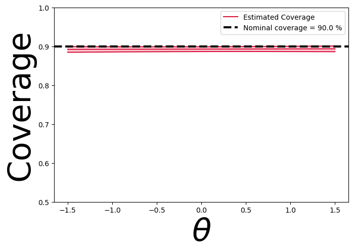
Coverage is approximately the correct level (90%) everywhere
coverage_probability_plot(
    parameters=parameters,
    coverage_probability=mean_proba,
    upper_proba=upper_proba,
    lower_proba=lower_proba,
    confidence_level=CONFIDENCE_LEVEL,
    param_dim=PARAM_DIM,
    figsize=(7.5, 5),
    ylims=(0.5, 1)
)
