%load_ext autoreload
%autoreload 2

Waldo Critical Values Construction

INTRO & SETTINGS

The goal of this tutorial is to show the capabilities of lf2i and Waldo with a simple example: inferring the mean \(\theta \in \mathbb{R}^{2}\) of a Gaussian model with fixed covariance, and a Gaussian prior distribution

\[\begin{split}\boldsymbol{\theta} \sim \mathcal{N}(\mathbb{0}, 0.1 \cdot \mathbb{I}), \\ \text{ } \mathbf{X}|\boldsymbol{\theta} \sim \mathcal{N}(\boldsymbol{\theta}, 0.01 \cdot \mathbb{I})\end{split}\]

In addition, we assume that we only observe one sample for each true \(\boldsymbol{\theta}\), i.e., \(n=1\).

For this tutorial, we leverage a posterior estimator (SNPE from the sbi library) as the main underlying inferential model.

# SETTINGS

LIKELIHOOD_COV = 0.01
PRIOR_LOC = 0
PRIOR_COV = 0.1

PARAM_DIM = 2
DATA_DIM = 2
BATCH_SIZE = 1  # assume we get to see only one observed sample for each “true” parameter
PARAM_SPACE_BOUNDS = {'low': -1.5, 'high': 1.5}  # a grid of points over [low, high]^(param_dim) is used to construct confidence sets

CONFIDENCE_LEVEL = 0.90

SIMULATE

Let’s start from the simulator, which is used internally to generate the data needed to

1. estimate the test statistics;

2. estimate the critical values; and

3. diagnose the constructed confidence regions

from lf2i.simulator.gaussian import GaussianMean

simulator = GaussianMean(
    likelihood_cov=LIKELIHOOD_COV,
    prior='gaussian',
    poi_space_bounds=PARAM_SPACE_BOUNDS,
    poi_grid_size=10_000,
    poi_dim=PARAM_DIM,
    data_dim=DATA_DIM,
    batch_size=BATCH_SIZE,
    prior_kwargs={'loc': PRIOR_LOC, 'cov': PRIOR_COV}
)

Observations

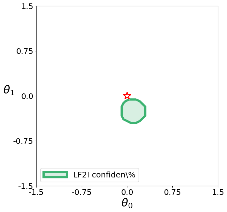
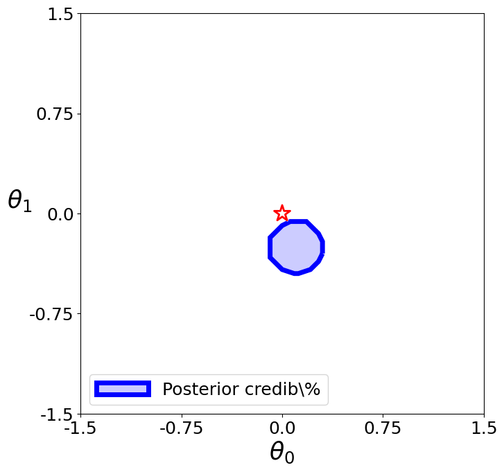
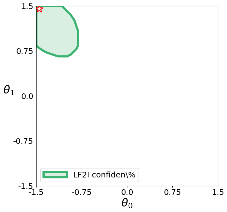
For simplicity, let’s use the simulator to generate two “observed” samples from the true likelihood: one consistent with the prior (\(\boldsymbol{\theta}^{\star} = [0, 0]\)) and one not (\(\boldsymbol{\theta}^{\star} = [-1.45, 1.45]\))

import torch

true_param_consistent, true_param_notconsistent = torch.Tensor([0, 0]), torch.Tensor([-1.45, 1.45])
observed_x_consistent = simulator.likelihood(true_param_consistent).sample(sample_shape=(BATCH_SIZE, ))
observed_x_notconsistent = simulator.likelihood(true_param_notconsistent).sample(sample_shape=(BATCH_SIZE, ))

CONFIDENCE SET by leveraging a POSTERIOR ESTIMATOR

Assume we want to do inference on the Gaussian mean by estimating its posterior distribution. Waldo allows to leverage a neural posterior estimator like SNPE to obtain a confidence region for the parameter of interest that is guaranteed to have the desired level of coverage regardless of

1. the consistency of the prior distribution with the data;

2. the true value of the parameter;

3. the size of the observed sample

The posterior estimator can be already trained or not. The example below assumes the estimator has not been trained yet, only instantiated up front.

Note: We require that posterior-based methods receive estimators whose interface matches one of AbstractNeuralPosterior or AbstractNeuralPosteriorTrainer from the lf2i.estimators.base_posteriors module.

from lf2i.inference import LF2I
from lf2i.test_statistics import Waldo
from lf2i.utils.other_methods import hpd_region
from lf2i.plot.parameter_regions import plot_parameter_regions

from sbi.inference import SNPE

/ocean/projects/mth260009p/jcarzon/conda/envs/tsi/lib/python3.11/site-packages/tqdm/auto.py:21: TqdmWarning: IProgress not found. Please update jupyter and ipywidgets. See https://ipywidgets.readthedocs.io/en/stable/user_install.html
  from .autonotebook import tqdm as notebook_tqdm

lf2i = LF2I(
    test_statistic=Waldo(
        estimator=SNPE(),
        estimation_method='posterior',
        poi_dim=PARAM_DIM,
        num_posterior_samples=20_000 # used to approximate conditional mean and variance of the Waldo test statistic
    )
)

Note that for this example we are using the simulator to obtain training datasets. If one has pre-simulated datasets, they can be given as inputs directly to the inference method.

confidence_region = lf2i.inference(
    x=torch.vstack((observed_x_consistent, observed_x_notconsistent)),
    evaluation_grid=simulator.poi_grid,
    confidence_level=CONFIDENCE_LEVEL,
    calibration_method='critical-values',
    calibration_model='nn',
    simulator=simulator,
    b=20_000, b_prime=10_000
)

Waldo Confidence Region

# The red star in the plot is the true parameter

plot_parameter_regions(
    confidence_region[0],
    param_dim=PARAM_DIM,
    true_parameter=true_param_consistent,
    param_names=['theta0', 'theta1'],
    parameter_space_bounds={'theta0': simulator.poi_space_bounds, 'theta1': simulator.poi_space_bounds},
    alpha_shape=True,  # contour,
    alpha=2,  # hyperparameter for contour (the lower, the more it converges to a convex hull)
    scatter=False,  # don't plot evaluation points
    figsize=(7.5, 7.5),
    colors=['mediumseagreen'],
    region_names=['LF2I confidence set']
)

/jet/home/jcarzon/probabilistic-regression/submodule/lf2i/src/lf2i/plot/parameter_regions.py:426: UserWarning: Contour might be unreliable if alpha is not chosen properly. Please plot scatter as well, and choose alpha appropriately (try from 1 to 20).
  warnings.warn("Contour might be unreliable if alpha is not chosen properly. Please plot scatter as well, and choose alpha appropriately (try from 1 to 20).")

Posterior Credible Region

plot_parameter_regions(
    hpd_region(
        posterior=lf2i.test_statistic.estimator,
        param_grid=simulator.poi_grid,
        x=observed_x_consistent,
        credible_level=CONFIDENCE_LEVEL
    )[1],
    param_dim=PARAM_DIM,
    true_parameter=true_param_consistent,
    param_names=['theta0', 'theta1'],
    parameter_space_bounds={'theta0': simulator.poi_space_bounds, 'theta1': simulator.poi_space_bounds},
    alpha_shape=True,  # contour,
    alpha=2,  # hyperparameter for contour (the lower, the more it converges to a convex hull)
    scatter=False,  # don't plot evaluation points
    figsize=(7.5, 7.5),
    colors=['blue'],
    region_names=['Posterior credible set']
)

/jet/home/jcarzon/probabilistic-regression/submodule/lf2i/src/lf2i/plot/parameter_regions.py:426: UserWarning: Contour might be unreliable if alpha is not chosen properly. Please plot scatter as well, and choose alpha appropriately (try from 1 to 20).
  warnings.warn("Contour might be unreliable if alpha is not chosen properly. Please plot scatter as well, and choose alpha appropriately (try from 1 to 20).")

Waldo Confidence Region

plot_parameter_regions(
    confidence_region[1],
    param_dim=PARAM_DIM,
    true_parameter=true_param_notconsistent,
    param_names=['theta0', 'theta1'],
    parameter_space_bounds={'theta0': simulator.poi_space_bounds, 'theta1': simulator.poi_space_bounds},
    alpha_shape=True,  # contour,
    alpha=2,  # hyperparameter for contour (the lower, the more it converges to a convex hull)
    scatter=False,  # don't plot evaluation points
    figsize=(7.5, 7.5),
    colors=['mediumseagreen'],
    region_names=['LF2I confidence set']
)

/jet/home/jcarzon/probabilistic-regression/submodule/lf2i/src/lf2i/plot/parameter_regions.py:426: UserWarning: Contour might be unreliable if alpha is not chosen properly. Please plot scatter as well, and choose alpha appropriately (try from 1 to 20).
  warnings.warn("Contour might be unreliable if alpha is not chosen properly. Please plot scatter as well, and choose alpha appropriately (try from 1 to 20).")

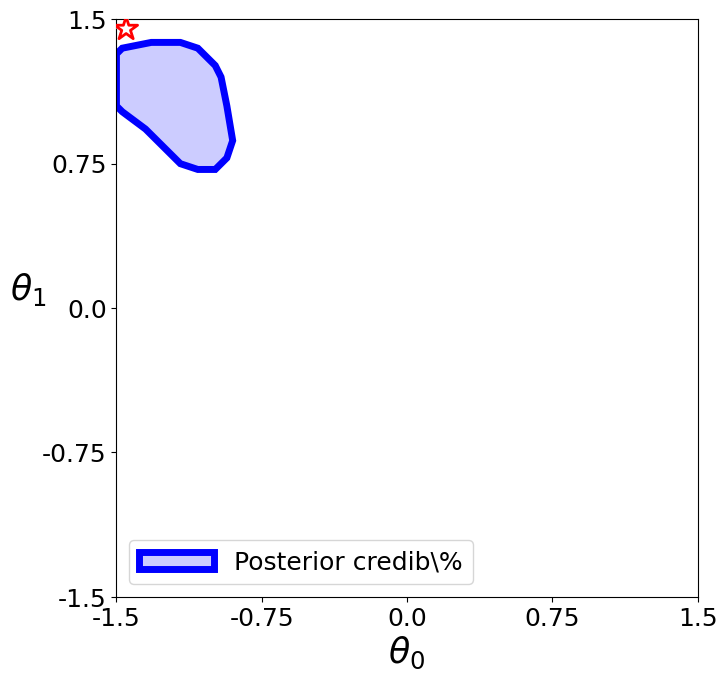
Posterior Credible Region

plot_parameter_regions(
    hpd_region(
        posterior=lf2i.test_statistic.estimator,
        param_grid=simulator.poi_grid,
        x=observed_x_notconsistent,
        credible_level=CONFIDENCE_LEVEL
    )[1],
    param_dim=PARAM_DIM,
    true_parameter=true_param_notconsistent,
    param_names=['theta0', 'theta1'],
    parameter_space_bounds={'theta0': simulator.poi_space_bounds, 'theta1': simulator.poi_space_bounds},
    alpha_shape=True,  # contour,
    alpha=2,  # hyperparameter for contour (the lower, the more it converges to a convex hull)
    scatter=False,  # don't plot evaluation points
    figsize=(7.5, 7.5),
    colors=['blue'],
    region_names=['Posterior credible set']
)

/jet/home/jcarzon/probabilistic-regression/submodule/lf2i/src/lf2i/plot/parameter_regions.py:426: UserWarning: Contour might be unreliable if alpha is not chosen properly. Please plot scatter as well, and choose alpha appropriately (try from 1 to 20).
  warnings.warn("Contour might be unreliable if alpha is not chosen properly. Please plot scatter as well, and choose alpha appropriately (try from 1 to 20).")

LOCAL COVERAGE

from lf2i.plot.coverage_diagnostics import coverage_probability_plot

Posterior Credible Regions

Note that for this example we are using the simulator to obtain training datasets. If one has pre-simulated datasets, they can be given as inputs directly to the inference method.

# this will take a few minutes because it has to compute a HPD credible region for each pair of (theta, x) in the simulated set
# the code is parallelized, but one can make it faster by decreasing the argument num_p_levels, which controls the number of level sets examined to construct the HPD region
# note that this might cause the credibility level of the HPD region to be only approximately equal to CONFIDENCE LEVEL
diagnostic_estimator, parameters, mean_proba, upper_proba, lower_proba, sizes = lf2i.coverage(
    region_type='posterior',
    simulator=simulator,
    b_double_prime=10_000,
    evaluation_grid=simulator.poi_grid.reshape(-1, PARAM_DIM),
    confidence_level=CONFIDENCE_LEVEL,
    posterior_estimator=lf2i.test_statistic.estimator,
    parameter_grid=simulator.poi_grid,
    exact=False,
    n_jobs=-2
)

Computing indicators for 10000 credible regions: 100%|██████████| 10000/10000 [02:42<00:00, 61.69it/s]

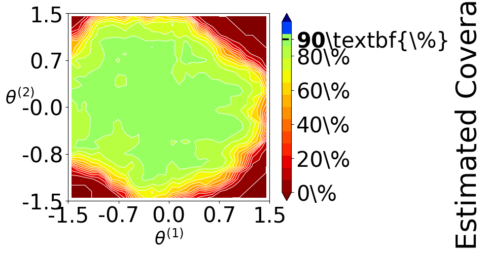
Coverage of posterior credible regions can be very erratic: they tend to overcover close to the “bulk” of the prior and severely undercover far from it. The correct level here is 90%

coverage_probability_plot(
    parameters=parameters,
    coverage_probability=mean_proba,
    upper_proba=None,
    lower_proba=None,
    confidence_level=CONFIDENCE_LEVEL,
    param_dim=PARAM_DIM,
    figsize=(12, 12)
)

Waldo Confidence Regions

Note that for this example we are using the simulator to obtain training datasets. If one has pre-simulated datasets, they can be given as inputs directly to the inference method.

diagnostic_estimator, parameters, mean_proba, upper_proba, lower_proba = lf2i.coverage(
    region_type='lf2i',
    confidence_level=CONFIDENCE_LEVEL,
    calibration_method='critical-values',
    simulator=simulator,
    b_double_prime=10_000,
    exact=False,
    n_jobs=-2
)

Approximating conditional mean and covariance for 10000 points...:   0%|          | 0/10000 [00:00<?, ?it/s]Approximating conditional mean and covariance for 10000 points...: 100%|██████████| 10000/10000 [03:11<00:00, 52.23it/s]

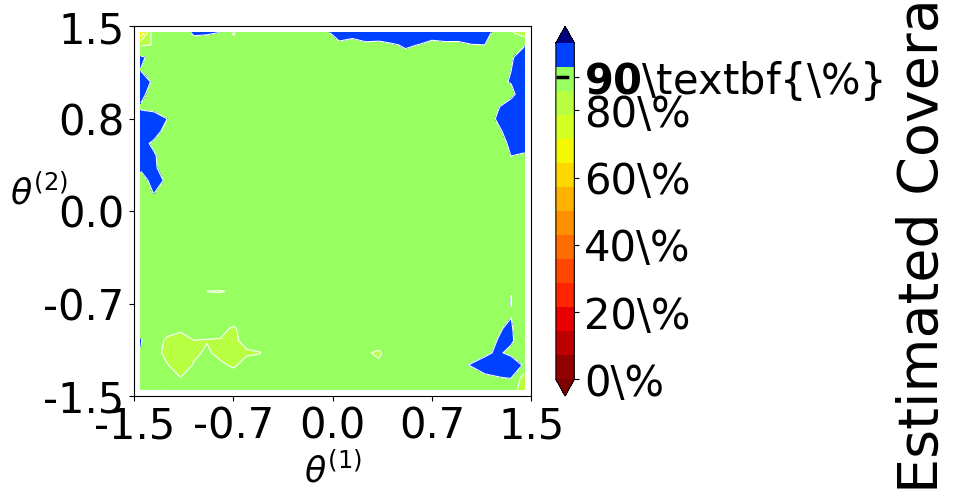
Coverage of Waldo is approximately 90% everywhere, as desired

coverage_probability_plot(
    parameters=parameters,
    coverage_probability=mean_proba,
    upper_proba=None,
    lower_proba=None,
    confidence_level=CONFIDENCE_LEVEL,
    param_dim=PARAM_DIM,
    figsize=(12, 12)
)