[1]:
%load_ext autoreload
%autoreload 2
Waldo Posterior P-value Construction
INTRO & SETTINGS
The goal of this tutorial is to show how to construct confidence sets for a generative-model-based test statistic, using both Waldo (posterior-based) and Posterior, calibrated via p-values (monotonic probabilistic classification), on a two-component Gaussian-mixture location model (as used in the MLST paper).
The likelihood is a two-component Gaussian mixture:
where the mixture weights and component scales are fixed. The parameter of interest is the location \(\theta\). As in the other tutorials, we leverage a posterior estimator (SNPE from the sbi library) as the main underlying inferential model — both Waldo (with estimation_method='posterior') and Posterior build on it, just using it differently to form the test statistic.
[2]:
# SETTINGS

POI_DIM = 1
DATA_DIM = 1
BATCH_SIZE = 1  # assume we get to see only one observed sample for each "true" parameter
POI_SPACE_BOUNDS = {'low': -2.0, 'high': 2.0}
POI_GRID_SIZE = 1_000

CONFIDENCE_LEVEL = 0.90

B = 20_000       # simulations to train the posterior estimator
B_PRIME = 10_000  # simulations to train the p-values calibration model
NUM_POSTERIOR_SAMPLES = 20_000
SIMULATE
[3]:
import torch

from lf2i.simulator.gmm import GaussianMixtureLocation

gmm = GaussianMixtureLocation(
    poi_space_bounds=POI_SPACE_BOUNDS,
    poi_grid_size=POI_GRID_SIZE,
    poi_dim=POI_DIM,
    data_dim=DATA_DIM,
    batch_size=BATCH_SIZE,
)
Observations
[4]:
x_obs = gmm(param=torch.tensor([[0.75]]), batch_size=1).reshape(1, DATA_DIM)
x_obs
[4]:
tensor([[0.8363]])
CONFIDENCE SET via Posterior + p-values
Posterior uses the (log-)posterior density itself as the test statistic. Calibrating it via calibration_method='p-values' fits a monotonic probabilistic classifier that estimates the rejection probability \(P(T \le \tau \mid \theta)\) directly, which doubles as a p-value function usable for confidence sets.
[5]:
from lf2i.inference import LF2I
from lf2i.test_statistics import Posterior
from sbi.inference import SNPE

posterior_ts = Posterior(poi_dim=POI_DIM, estimator=SNPE())
lf2i_posterior = LF2I(test_statistic=posterior_ts)

posterior_region = lf2i_posterior.inference(
    x=x_obs,
    evaluation_grid=gmm.poi_grid.reshape(-1, 1),
    confidence_level=CONFIDENCE_LEVEL,
    calibration_method='p-values',
    calibration_model='nn',
    simulator=gmm,
    b=B,
    b_prime=B_PRIME,
)
/ocean/projects/mth260009p/jcarzon/conda/envs/tsi/lib/python3.11/site-packages/tqdm/auto.py:21: TqdmWarning: IProgress not found. Please update jupyter and ipywidgets. See https://ipywidgets.readthedocs.io/en/stable/user_install.html
  from .autonotebook import tqdm as notebook_tqdm
Estimating test statistic ...
/ocean/projects/mth260009p/jcarzon/conda/envs/tsi/lib/python3.11/site-packages/sbi/neural_nets/net_builders/flow.py:149: UserWarning: In one-dimensional output space, this flow is limited to Gaussians
  x_numel = get_numel(
 Neural network successfully converged after 44 epochs.
Calibration ...
Evaluating posterior for 10000 points ...: 100%|██████████| 10000/10000 [02:45<00:00, 60.42it/s]
Retraining calibration...
  [calibration] CDF estimator — augment_kwargs ignored.
  [calibration] CDF estimator: fitting on 10000 raw (T, θ) pairs.

Constructing confidence sets ...
Evaluating posterior for 1 points ...: 100%|██████████| 1/1 [01:51<00:00, 111.04s/it]
Computing p-values...

Creating set 0...
CONFIDENCE SET via Waldo (posterior-based) + p-values
Waldo with estimation_method='posterior' instead centers the test statistic on the posterior mean and variance (estimated from posterior samples), rather than the density itself — a different way of using the same underlying posterior estimator to build a confidence set.
[6]:
from lf2i.test_statistics import Waldo

waldo_ts = Waldo(
    estimator=SNPE(),
    poi_dim=POI_DIM,
    estimation_method='posterior',
    num_posterior_samples=NUM_POSTERIOR_SAMPLES,
)
lf2i_waldo = LF2I(test_statistic=waldo_ts)

waldo_region = lf2i_waldo.inference(
    x=x_obs,
    evaluation_grid=gmm.poi_grid.reshape(-1, 1),
    confidence_level=CONFIDENCE_LEVEL,
    calibration_method='p-values',
    calibration_model='nn',
    simulator=gmm,
    b=B,
    b_prime=B_PRIME,
)
Estimating test statistic ...
 Neural network successfully converged after 47 epochs.
Calibration ...
Approximating conditional mean and covariance for 10000 points...: 100%|██████████| 10000/10000 [09:56<00:00, 16.75it/s]
Retraining calibration...
  [calibration] CDF estimator — augment_kwargs ignored.
  [calibration] CDF estimator: fitting on 10000 raw (T, θ) pairs.

Constructing confidence sets ...
Approximating conditional mean and covariance for 1 points...: 100%|██████████| 1/1 [00:00<00:00, 7.58it/s]
Computing p-values...

Creating set 0...
COMPARISON
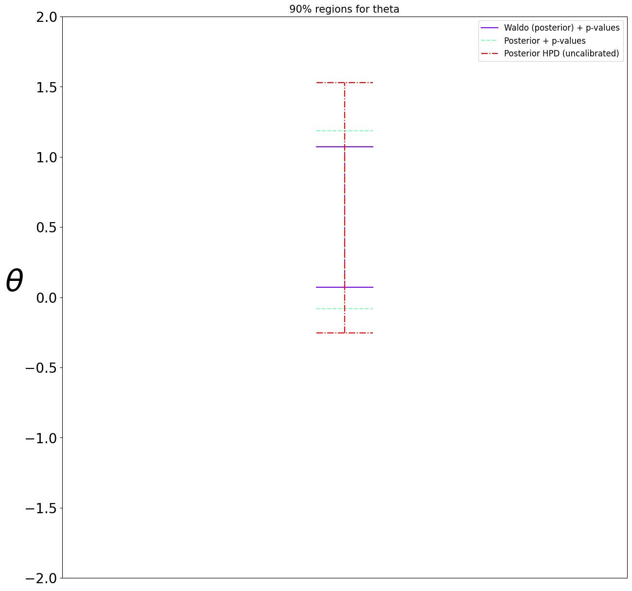
Alongside the two LF2I-calibrated regions, we also plot the posterior’s own highest-posterior-density (HPD) credible region at the same level, as an (uncalibrated) reference.
[7]:
from lf2i.utils.other_methods import hpd_region
from lf2i.plot.parameter_regions import plot_parameter_regions

_, hpd_set = hpd_region(
    posterior=posterior_ts.estimator,
    param_grid=gmm.poi_grid.reshape(-1, 1),
    x=x_obs,
    credible_level=CONFIDENCE_LEVEL,
)

plot_parameter_regions(
    waldo_region[0], posterior_region[0], hpd_set,
    param_dim=POI_DIM,
    parameter_space_bounds=POI_SPACE_BOUNDS,
    region_names=['Waldo (posterior) + p-values', 'Posterior + p-values', 'Posterior HPD (uncalibrated)'],
    title=f'{int(CONFIDENCE_LEVEL*100)}% regions for theta',
)